A tutorial on binary descriptors – part 4 – The BRISK descriptor

This fourth post in our series about binary descriptors that will talk about the BRISK descriptor [1]. We had an introduction to patch descriptors, an introduction to binary descriptors and posts about the BRIEF [2] and the ORB [3] descriptors.

We’ll start by showing the following figure that shows an example of using BRISK to match between real world images with viewpoint change. Green lines are valid matches, red circles are detected keypoints.

BRISK descriptor – example of matching points using BRISK

As you may recall from the previous posts, a binary descriptor is composed out of three parts:

1. A sampling pattern: where to sample points in the region around the descriptor.
2. Orientation compensation: some mechanism to measure the orientation of the keypoint and rotate it to compensate for rotation changes.
3. Sampling pairs: which pairs to compare when building the final descriptor.

Recall that to build the binary string representing a region around a keypoint we need to go over all the pairs and for each pair (p1, p2) – if the intensity at point p1 is greater than the intensity at point p2, we write 1 in the binary string and 0 otherwise.

The BRISK descriptor is different from the descriptors we talked about earlier, BRIEF and ORB, by having a hand-crafted sampling pattern. BRISK sampling pattern is composed out of concentric rings:

BRISK descriptor – BRISK sampling pattern

When considering each sampling point, we take a small patch around it and apply Gaussian smoothing. The red circle in the figure above illustrations the size of the standard deviation of the Gaussian filter applied to each sampling point.

Short and long distance pairs

When using this sampling pattern, we distinguish between short pairs and long pairs. Short pair are pairs of sampling points that their distance is below a certain threshold d_max and long pairs are pairs of sampling points that their distance is above a certain different threshold d_min, where d_min>d_max, so there are no short pairs that are also long pairs.

Long pairs are used in BRISK to determine orientation and short pairs are used for the intensity comparisons that build the descriptor, as in BRIEF and ORB. The

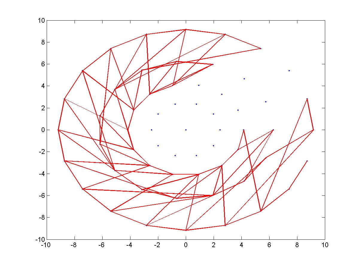
To illustrate this and help make things clear, here are figures of BRISK’s short pairs – each red line represent one pair. Each figure shows 100 pairs:

BRISK descriptor – BRISK short pairs

BRISK descriptor – BRISK short pairs

BRISK descriptor – BRISK’s short pairs

BRISK descriptor – BRISK’s short pairs

BRISK descriptor – BRISK’s short pairs

Computing orientation

BRISK is equipped with a mechanism for orientation compensation; by trying to estimate the orientation of the keypoint and rotation the sampling pattern by that orientation, BRISK becomes somewhat invariant to rotation.

For computing the orientation of the keypoint, BRISK uses local gradients between the sampling pairs which are defined by

BRISK descriptor – local gradients forumla

Where g(pi,pj) is the local gradient between the sampling pair (pi,pj), I is the smoothed intensity (by a Gaussian) in the corresponding sampling point by the appropriate standard deviation (see the figure above of BRISK sampling pattern).

To compute orientation, we sum up all the local gradients between all the long pairs and take arctan(gy/gx) – the arctangent of the the y component of the gradient divided by the x component of the gradient. This gives up the angle of the keypoint. Now, we only need to rotate the short pairs by that angle to help the descriptor become more invariant to rotation. Note that BRISK only use long pairs for computing orientation based on the assumption that local gradients cancel each other thus not necessary in the global gradient determination.

Building the descriptor and descriptor distance

As with all binary descriptors, building the descriptor is done by performing intensity comparisons. BRISK takes the set of short pairs, rotate the pairs by the orientation computed earlier and makes comparisons of the form:

BRISK descriptor – Intensity comparisons

Meaning that for each short pair it takes the smoothed intensity of the sampling points and checked whether the smoothed intensity of the first point in the pair is larger than that of the second point. If it does, then it writes 1 in the corresponding bit of the descriptor and otherwise 0. Remember that BRISK uses only the short pairs for building the descriptor.

As usual, the distance between two descriptors is defined as the number of different bits of the two descriptors, and can be easily computed as the sum of the XOR operator between them.

You probably ask what about performance. Well we’ll have a detailed post that will talk all about performance of the different binary descriptors, but for now I will say a few words comparing BRISK to the previous descriptors we talked about – BRIEF and ORB:

• BRIEF outperforms BRISK (and ORB) in photometric changes – blur, illumination changes and JPEG compression.
• BRISK slightly outperforms BRIEF in viewpoint changes, but performs about the same as ORB in overall.

Stay tuned for the next post in the series that will talk about the FREAK descriptor, the last binary descriptor we will focus on before giving a detailed performance evaluation.

Gil.

References:

[1] Leutenegger, Stefan, Margarita Chli, and Roland Y. Siegwart. “BRISK: Binary robust invariant scalable keypoints.” Computer Vision (ICCV), 2011 IEEE International Conference on. IEEE, 2011.‏

[2] Calonder, Michael, et al. “Brief: Binary robust independent elementary features.” Computer Vision–ECCV 2010. Springer Berlin Heidelberg, 2010. 778-792.‏

[3] Rublee, Ethan, et al. “ORB: an efficient alternative to SIFT or SURF.” Computer Vision (ICCV), 2011 IEEE International Conference on. IEEE, 2011.‏